A Study on the Prediction of Real-Time Bead Width Using a DNN Algorithm in Tandem GMA Welding
Abstract
The tandem welding method employs multiple wires to enhance productivity and increase deposition rates in arc welding. This study aimed to develop and validate a deep neural network (DNN) algorithm for predicting bead geometry. The algorithm processes real-time data and bead geometry measurements obtained from tandem gas metal arc (GMA) welding. A tandem GMA welding experiment with SS400 plates was performed, collecting current and voltage waveforms in real-time via a monitoring system. Furthermore, post-experiment bead width and height data were precisely captured with a 3D scanner. The acquired data served as training data to develop the DNN algorithm. Backpropagation was employed in the DNN for bead geometry prediction; its accuracy was evaluated using the Predictive Ability of Model (PAM). The DNN algorithm achieved over 96% accuracy in predicting bead width and height, suggesting its applicability in industrial settings like shipyards and automotive plants to improve weld quality and efficiency.
Keywords:
Tandem GMA welding, Bead geometry, DNN algorithm, BP algorithm, Real-time monitoring1. Introduction
Welding is a crucial process that determines the final products and productivity in shipbuilding, automobiles, and machinery. In various welding processes, arc welding is a process that generates an arc using high-energy sources such as electricity to melt the materials to integrate parts. The process monitoring of arc welding employs multiple types of sensors, collects real-time data, and analyzes it systematically. Generally, current and voltage sensors are used to measure the significant effect of arc stability and metal transfer on welding quality, after which the collected data are synchronized for analysis[1-2]. Studies have been conducted to evaluate and ensure the quality of joint using real-time welding process monitoring. These studies used collected data, the mean and standard deviation of welding process variables, and short circuit frequencies. Adolfsson et al.[3]; analyzed the averages, standard deviations, and variances of welding current, arc voltage signal, frequency, and duration of short circuits to evaluate welding quality. In an effort to estimate the amount of spatter in the short circuit transfer mode of GMA welding, Kang et al.[4] attempted to develop statistical models. The bead geometry is a representation that can be used to assess the quality of the joint. Therefore, it is crucial to ensure an appropriate bead geometry However, obtaining high-quality bead geometry through experiments is time-consuming and costly because the welding process is complex, with multiple inputs and outputs, and interrelated process variables that affect bead geometry. Therefore, studies have been conducted to develop a prediction model that uses the relationship between current and voltage as input variables and bead geometry as the output variable. Numerical analysis is effective method to predict the bead geometry using process variables[5-7]. However, because of the nonlinear process, the accuracy of a simplified numerical model for predicting bead geometry is not accuracy. The accuracy of regression analysis-based predictive models is typically high within an experiment. Kim et al.[8] used regression analysis to determine the relationship between process variables and bead geometry in GMA welding. Recently, deep learning has been used to develop a predictive model for bead geometry. Jin et al. [9] studied the prediction of back bead in GMAW using deep learning. Di et al.[10]; proposed neural-network-based selforganized fuzzy logic control for arc welding. Kim et al.[11]; chose a backpropagation(BP) neural network to predict a bead geometry for the GMA welding. Ge et al.[12] collected data on welding defects, used an auto-regressive(AR) model to analyze errors, and applied the hidden Markov model algorithm for real-time identification and prediction of defects. Recently, studies have been conducted on improving welding productivity. The simplest way to enhance welding productivity is by increasing welding speed or modifying welding methods. With this reason, the tandem GMA, a multi-electrode welding process, has recently been examined[13-15].
Although the tandem GMA process has high productivity because it leads to a single weld pool using two or more welding torches and wire, there are challenges in ensuring joint quality because defects can occur due to the proximity of two or more welding arcs[16-17]. Recently, various analytical and experimental tests have been conducted on the tandem welding process. However, there is a scarcity of studies that accurately predict bead geometry for tandem GMA. Particularly, the development of a prediction algorithm for bead geometry using real-time welding data has not yet been performed. Therefore, the tandem GMA welding of SM490 steel was conducted, whereby the welding current and voltage were monitored and collected in real-time in this study. The width and height of the beads were measured accurately using a 3D scanner. A prediction model based on neural networks was developed using the data obtained from real-time tandem GMA welding. The real-time data was used to train the DNN algorithm that predicts bead geometry using the BP learning technique. In addition, the accuracy of the developed bead geometry prediction algorithm was validated using Predictive Ability of Model(PAM).
2. Experimental work
2.1 Material and apparatus
Table 1 shows the chemical properties of the base material utilized in this experiment, specifically SM490, which had a thickness of 9 mm.

Chemical composition of SM490(mass%)
Tandem welding is a welding process that uses two or more independent power sources and torches. It is classified into leading and trailing welding. The tandem GMA welding apparatus for this study consists of a welding robot, two welding power sources, and a monitoring system, as shown in Fig. 1. The OTC Welbee P500L, a DC pulse welding power source, was used in constant voltage mode as the primary power source, whereas the OTC DW300 was used in AC pulse mode as the secondary power source. A Yaskawa AR700 welding robot was used for GMA welding. A 1.2-mm-diameter solid wire(AWS: A5.18 ER70S-6) and a 1.2-mm-diameter flux-cored wire(AWS: A5.20: E71T-1C) were used for leading and trailing welding, respectively. An Ar 80% + CO2 20% and Ar 90% + CO2 10% mixed gas was supplied at 18 L/min and 21 L/min for the lead and trailing welding, respectively. The welding was performed with bead-on-plate. The welding monitoring system (WET-300A) from Monitek was used to monitor the real-time process data. To achieve this, a hall sensor-type welding current and voltage sensor was installed. Measured data was recorded at a rate of 2.5 kHz/s and stored on a personal computer.

Experimental setup for tandem GMA welding
2.2 Experimental design
As shown in Fig. 2, the input variables were welding current and voltage, while the output variables were bead width and height. The full factorial design was used as the experimental design. In the full factorial design, each input variable is arranged at regular intervals, and experiments are conducted for all combinations of all levels. The input variables and their levels are listed in Table 2. The welding current and welding voltage were adjusted from 230 A and 15 V to 270 A and 35 V, respectively. Other variables, such as the torch angle (90o), welding speed of 1.6 m/min, contact tip to work distance of 18 mm, and shielding gas flow rate, were kept constant.

Input and output variables of the tandem GMA welding
Tandem GMA welding variables and their levels
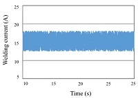
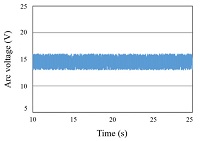
Table 3 shows the results from the experiments based on different welding conditions, including the welding current and voltage, which were collected in real time.
Result of experimental works: Bead geometry, welding current, and welding voltage
2.3 Measurement of bead width and length
In the past, the geometry of beads was measured manually using tools like calipers. However, these methods were time-consuming and lacked accuracy. Therefore, a high-resolution non-contact 3D scanner, the Creaform Handyscan 700, was used to accurately measure the width and length of the beads. The measurement values were obtained as 3D mesh data, allowing for modeling of the bead geometry, as shown in Fig. 3.

The measured bead geometry using a 3D scanner
3. Results and discussion
3.1 Development of BP-based DNN algorithm
An artificial neural network(ANN) is constructed based on the human nervous system. The ANN is composed of an input layer, a hidden layer, and an output layer, with each layer comprising multiple nodes. Training data(features) entered into each node in layers are multiplied by weights randomly set between nodes in an input and output layer. After bias is added, training data enters each node in a hidden layer. It then undergoes various activation functions that return output values. The output values of each node, computed as such, are entered into the next hidden layer and undergo the same process. They enter into the last output layer, and the provisional output, whose difference with the actual value (label) is determined by the loss function, is computed. Fundamentally, once the feedforward propagation process is completed, backpropagation is performed to reduce the error determined by the loss function. Backpropagation operates in the reverse direction of feedforward propagation, with the optimization algorithm sequentially adjusting the weights and biases of the nodes using partial derivatives. The ANN performs feedforward and backpropagation cycles until a set number of iterations or conditions are met. ANNs are categorized into single-layer perceptron, multi-layer perceptron, and deep neural networks(DNNs) with two or more hidden layers, based on their development stages. While traditional ANNs can handle simple data such as the XOR problem, they cannot overcome the vanishing gradient problem or overfitting when the number of hidden layers increases[18-19]. DNN is a deep learning model. The major difference between general neural networks and DNN is the number of hidden layers, and as shown in Fig. 4, there are multiple hidden layers between the input and output layers. Since DNNs comprise more layers than ANNs, they often require more training data to obtain better results than ANNs.

A typical architecture of DNN
The DNN is trained using the backpropagation algorithm, and due to the extensive computations, its ability to review all datasets when gradient descent is applied is slowed down. Therefore, stochastic gradient descent is applied, which calculates the gradient using only a subset of the data randomly drawn from the full dataset. Weights are adjusted based on stochastic gradient descent in Eq. (1).
| (1) |
Here, η and C represent the learning rate and cost function, respectively. The loss function, also known as the cost function, quantifies and minimizes the difference between the predicted values and the actual data during training. Several activation functions, including Sigmoid and Tanh, are available when designing a hidden layer. Softmax and cross-entropy functions are used as activation and cost functions in a multi-class classification task. The softmax function is defined by Eq. (2).
| (2) |
Here, Pj is class probability, while xj and xk represent the total input of each unit j and the total input of unit k, respectively. Cross-entropy is defined by Eq. (3).
| (3) |
Here, dj is the target probability for output j and Pj is the probability output for j after applying the corresponding activation function. The number of neurons in a hidden layer of the DNN undergoes a trial-and-error method. To improve the overall accuracy of the neural network, the training was continued until the target error values were reached, the maximum number of epochs were completed, or X reached its maximum value[13].
Table 4 shows the testing of three to ten hidden layers to determine the optimal number of neurons for training the DNN algorithm. Out of 200,000 samples, 199,900 were used for training and 100 were used for testing the prediction of a bead geometry.
Setpoint for DNN training
Fig. 5 compares actual and predicted values of bead widths according to the changes in the number of neurons in a hidden layer. When a hidden layer had seven neurons, the correlation coefficient R was 0.98911, near 1, which indicates that the model accurately predicted bead widths.

R-value for the DNN configuration between 3 and 10 neurons in the hidden layer on bead width
As a loss function, the mean squared error(MSE) is the average of the squared differences between the actual and predicted values for the entire dataset, and MSE is defined as in Eq. (4).
| (4) |
Here, Yi is the experimental value, is the predicted value, and n is the number of experiments.
The closer the MSE is to 0, the higher the accuracy of the predicted values. Table 5 and Fig. 6 show the MSE error of values predicted by the DNN algorithm and training values. If there are seven neurons in a hidden layer, the MSEs of the test and training data are 0.1153 and 0.1034, respectively, indicating that the model accurately predicts bead widths.
MSE values for DNN configuration for bead width with hidden layer

MSE values for DNN configuration for bead width
The algorithm was trained to minimize the error by adjusting the number of neurons in the initial hidden layer from three to ten in order to develop a bead height prediction algorithm. Fig. 7 shows the results comparing the actual and predicted values of bead heights according to the number of neurons in a hidden layer. The correlation coefficient R was closest to 1 at 0.98992; when a hidden layer had eight neurons, confirming that it accurately predicted bead heights.

R-value for the deep neural network configuration between 3 and 10 neurons in the hidden layer for bead height
Table 6 and Fig. 8 show the MSE errors of values predicted by the DNN algorithm and training data. When there were seven neurons in a hidden layer, the MSEs of the test and training data were 0.1153 and 0.1034, respectively. The minimal error confirmed that the bead widths were accurately predicted. Table 6. MSE values for deep neural network configuration between 3 and 10 neurons in the hidden layer for bead height.
MSE values for DNN configuration for bead height with hidden layer

MSE values for DNN configuration for bead height
3.2 Evaluation of the BP-based DNN algorithm
The accuracy of the developed BP-based DNN algorithm in predicting bead width and height was evaluated using the PAM in Eq. (5)[20].
| (5) |
Here, NPAM represents the number of predicted values in the range . Ntotal is the total number of predicted values, BM is the actual value, and BP is the value predicted by the algorithm. The standard deviation describes the model distribution and indicates how closely the model predicts the measured bead width. whereas PAM accurately assesses predictions within an error range of 10% and measures the accuracy of the model. The prediction accuracy was performed by comparing the measured and predicted bead, as shown in Fig. 9 and 10. Fig. 11 and 12 show the number of errors, and the prediction accuracy of the developed algorithm was computed at 96% for both bead widths and heights, as shown in Table 7. The error range within 10% confirmed that the developed algorithm predicts bead geometry accurately.

The predicted results using BP-based DNN algorithm for bead width

The predicted results using BP-based DNN algorithm for bead height

Comparison between the measured and predicted bead width from the developed BP-based DNN algorithm

Comparison between the measured and predicted bead height from the developed BP-based DNN algorithm
Performance of the developed DNN algorithm for bead geometry
4. Conclusion
In this study, tandem GMA welding was performed on a bead-on-plate using SM490 to develop a bead geometry prediction algorithm. The bead geometry prediction algorithm was developed using real-time data, leading to the following conclusions:
(1) The Tandem GMA welding experiment was performed 25 times for each welding condition, following the full factorial experimental method. Real-time data on welding current and voltage waveforms were collected during the welding process. Furthermore, an accurate measurement of the bead width and height was obtained using a 3D scanner as the output variables. The bead geometry prediction algorithm was developed using real-time data and measured data from 3D modeling.
(2) The number of hidden layer neurons was determined by the BP algorithm, which is the structure of the DNN algorithm. As a result, the correlation coefficient of bead widths R was 0.98911 when the hidden layer had seven neurons. For bead heights, R was 0.98992 when a hidden layer had eight neurons, indicating an optimal number of neurons.
(3) To confirm the reliability of the backpropagation (BP)-based DNN algorithm, the algorithm's predicted values were compared and analyzed with the measured values using PAM. As a result, the prediction accuracy of the developed algorithm was 96% for both bead width and height, confirming the efficiency of the developed BP-based DNN algorithm.
(4) The developed BP-based DNN algorithm can improve the quality and productivity of tandem welding of steel plates, which constitutes 70% of all welding processes.
Acknowledgments
This research was supported by the Korea Institute of Industrial Technology (KITECH) under one of its major projects, “Development of Smart Welding System Modules with Dynamic Variable Control for Full Penetration Weld (KITECH EH-23-0007)
References
-
Kim, I. S., Son, J. S., Yarlagadda, P. K. D. V., 2003, A Study on the Quality Improvement of Robotic GMA Welding Process, Robot. Comput.-Integr. Manuf., 19:6 567-572.
[https://doi.org/10.1016/S0736-5845(03)00066-8]

-
Kim, Y. M., Chun, H. P., 2023, Recent Research Trend of Arc Welding Quality Monitoring Technology in Korea, J. Weld. Join., 41:2 81-89.
[https://doi.org/10.5781/JWJ.2023.41.2.1]
- Adolfsson, S., Bahrami, A., Bolmsjo, G., Claesson, I., 1999, On-Line Quality Monitoring in Short-Circuit Gas Metal Arc Welding, Weld. J., 78:2 59-73.
- Kang, M. J., Rhee, S., 2001, The Statistical Models for Estimating the Amount of Spatter in the Short Circuit Transfer Mode of GMAW, Welding Research Supplement, 80:1 1-8.
-
Sripriyan, K., Ramu, M., Thyla, P. R., Anantharuban, K., Karthigha, M., 2022, Characteristic of Weld Bead using Flat Wire Electrode in GMAW Inline during the Process: An Experimental and Numerical Analysis, Int. J. Pressure Vessels Pip., 196 104623.
[https://doi.org/10.1016/j.ijpvp.2022.104623]
-
Rao, K.V., Parimi, S., Raju, L. S., Suresh, G., 2022, Modelling and Optimization of Weld Bead Geometry in Robotic Gas Metal Arc-based Additive Manufacturing using Machine Learning, Finite-element Modelling and Graph Theory and Matrix Approach, Soft Comput., 26 3385-3399.
[https://doi.org/10.1007/s00500-022-06749-x]
-
Wu, Y., Wang, J., Xu, G., Jing, Y., 1999, Numerical Analysis Modeling of Temperature Field in Swing-arc Narrow Gap GMA Welding with Additional Wire, Int. J. Adv. Manuf. Technol., 125 1559-1576.
[https://doi.org/10.1007/s00170-022-10772-5]
-
Lee, B. R., Oh, W. B., Kim, H. H., Jeong, Y. J., Yoon, J. S., Kim, I. S., 2001, A Study on the Cluster-wise Regression Model for Bead Width in the Automatic GMA Welding, International Conference on Information Networking, 22683109.
[https://doi.org/10.1109/ICOIN56518.2023.10049016]
-
Jin, C. N., Shin, S. M., Yu, J. Y., Rhee, S. H., 2020, Prediction Model for Back-Bead Monitoring During Gas Metal Arc Welding Using Supervised Deep Learning, IEEE Access, 8 20191413.
[https://doi.org/10.1109/ACCESS.2020.3041274]
-
Di, L., Srikanthan, T., Chandel, R. S., Katsunori, I., 2001, Neural-network-based Self-organized Fuzzy Logic Control for Arc Welding, Eng. Appl. Artif. Intell., 14:2 115-124.
[https://doi.org/10.1016/S0952-1976(00)00057-9]
-
Kim, M. S., Shim, S. M., Kim, D. H., Rhee, S., 2020, A Study on the Algorithm for Determining Back Bead Generation in GMA Welding using Deep Learning, J. Weld. Join., 36:2 74-81.
[https://doi.org/10.5781/JWJ.2018.36.2.11]
-
Ge, M., Du, R., Xu, Y., 2004, Hidden Markov Model based Fault Diagnosis for Stamping Processes, Mech. Syst. Signal. Process., 18:2 391-408.
[https://doi.org/10.1016/S0888-3270(03)00076-1]
-
Wu, D. S., Huang, J. L., Kong, L., Hua, X. M., Wang, M., Li, H., Liu, S. T., 2023, Numerical Analysis of Arc and Molten Pool Behaviors in High Speed Tandem TIG Welding of Titanium Tubes, Transactions of Nonferrous Metals Society of China, 33:6 1768-1778.
[https://doi.org/10.1016/S1003-6326(23)66220-X]
-
Qin, G., Feng, C., Ma, H., 2021, Suppression Mechanism of Weld Appearance Defects in Tandem TIG Welding by Numerical Modeling, J. Mater. Res. Technol., 14 160-173.
[https://doi.org/10.1016/j.jmrt.2021.06.042]
-
Kam, D. H., Lee, T. H., Kim, D.Y., Kim, J. D., Kang, M. J., 2021, Weld Quality Improvement and Porosity Reduction Mechanism of Zinc Coated Steel using Tandem Gas Metal Arc Welding (GMAW), J. Mater. Process. Technol., 294 117127.
[https://doi.org/10.1016/j.jmatprotec.2021.117127]
-
Park, C. K., Lee, J. P., Park, M. H., Kim, I. S., 2015, A Study on the Performance Evaluation of the Welded Joint to Maintain the Quality of the Tandem GMAW, Journal of the Korean Society of Marine Engineering, 39:3 230-237.
[https://doi.org/10.5916/jkosme.2015.39.3.230]
-
Kang, S. H., Bang, H. S., Kim, C. H., 2018, Spatter Generation During Constant Voltage DC-AC Pulse Tandem Gas Metal Arc Welding Process, J. Weld. Join., 36:3 65-71.
[https://doi.org/10.5781/JWJ.2018.36.3.10]
-
Widrow, B., Lehr, M. A., 1990, 30 Years of Adaptive Neural Networks: Perceptron, Madaline, and Backpropagation, Proc. IEEE, 78:9 1415-1442.
[https://doi.org/10.1109/5.58323]
- Minsky, M., Papert, S. A., 1969, Perceptrons : An Introduction to Computational Geometry, MIT Press, MA.
-
Lee, B. R., Kim, H. H., Jeong, Y. J., Oh, W. B., Kim, I. S., 2022, A Study on the Real-Time Prediction of the Surface Roughness during the Cutting Process using an ANN Algorithm, Trans. Korean Soc. Mech. Eng. A, 46:12 1023-1031.
[https://doi.org/10.3795/KSME-A.2022.46.12.1023]

Senior Researcher in the Department Maritime Technology Verification Research Team, Korea Marine Equipment Research Institute.
His research interest is Arc Welding Process.
E-mail: wboh@komeri.re.kr

Senior Researcher in the Carbon&Light Materials Application R&D Group, Korea Institute of Industrial Technology.
Her research interest is Welding and Joining.
E-mail: shimjy@kitech.re.kr